Colored Noise: Frequency-Domain Filtering
Noise signals that display specific frequency spectra are attributed colors, an allusion to the color of visible light showing the same. Like white light, white noise has uniform power spectral density, containing the same power in all frequency intervals. Pink noise has a power spectral density inversely proportional to frequency, showing a \(1/f\) spectrum and a pinkish hue in the visible spectrum. Brown(ian) noise is named as such because it’s the product of Brownian motion, but actually, it is colored red due to its amplified low-frequency content.
Methods to generate colored noise sources for time-domain simulations generally involve generating white noise and using a filter to produce the desired spectrum. Some of these time-domain filters can be trivial to build. A simple accumulator will be enough to approximate the \(1/f^2\) spectra. However, synthesizing time-domain filters that produce \(1/f\) spectra is much less trivial. Generally, filter stages show 20 dB/dec response, and it’s not clear how to combine these to build the 10 dB/dec spectra of pink noise.
This post presents a method that uses frequency-domain processing to generate colored noise sources to avoid this challenge altogether [1]. The idea is to manipulate the white noise signal to the desired shape in the frequency domain via a shaping function. The discrete Fourier transform (DFT) and its inverse are used to bring the signal back and forth, and all the processing is done in the frequency domain. The method presented is supposed to be a precursor to an post tackling the challenge of developing time-domain filters to generate \(1/f\) noise.
The Method
The algorithm for frequency domain filtering is quite straightforward. Take the DFT of a white noise signal to get its frequency domain representation, multiply it with the desired shaping function, and use the IDFT to return the signal to the time domain. Using Python and NumPy, it can be implemented as follows:
def generateColoredNoise(n_pts: int,
                         exp: float
                         ) -> NDArray[Shape['Any'], ComplexFloating]:
    # generate white noise with 0 mean
    x = np.random.randn(n_pts)
    x = x - np.mean(x)

    # generate the shaping function for the desired exponent
    f = generateShapingFunction(n_pts, exp)

    # frequency domain filtering
    x_f = np.fft.fft(x)
    y_f = x_f*f
    y = np.fft.ifft(y_f)
    return y
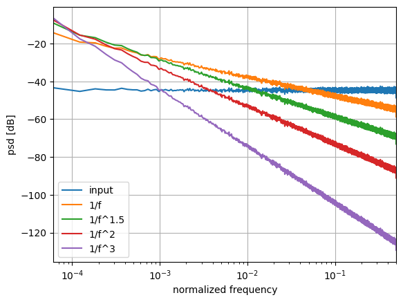
Running the above a few times and averaging the results shows the expected frequency-domain shape for different exponents. In the figure below, noise for each exponent was generated for 1000 runs and the magnitude of their outputs was averaged to show their spectra clearly. The signals have also been scaled to have the same approximate power, which makes them easy to compare in the time domain.
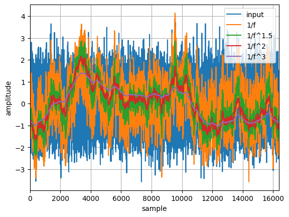
The figure below shows one of the runs in the time domain. Because of the scaling, the signals with the higher exponents tend to show much less high-frequency content and have approximately the same magnitude.
The only missing piece of the puzzle is generating the shaping function.
The Shaping Function
DFTs of real signals are symmetric around the Nyquist frequency. This property has to be maintained after shaping in the frequency domain to generate real, time-domain signals. The implication is that the shaping function must also be symmetric around \(f_s/2\). The function below generates these shaping functions for different powers of \(1/f\).
def generateShapingFunction(n_pts: int,
                            exp: float
                            ) -> NDArray[Shape['Any'], Float]:
    f = np.ones(n_pts)
    for i in range(1, int(n_pts/2)+1):
        f[i] = 1/i**(exp/2)
        f[n_pts-i] = f[i]

    return f
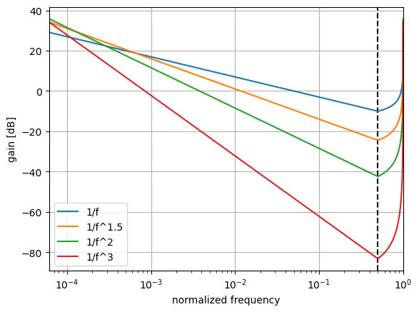
The figure below shows the gain of the generated functions in log-log space. The different slopes correspond to different exponents. The dashed line shows the Nyquist frequency, and the functions are symmetric with respect to it.
If this property were not satisfied, the resulting output of the IDFT would have significant imaginary content. Since the goal is to generate real-valued noise signals, this is undesirable. We can discard the imaginary component of the signal, but removing this data would make the magnitude response deviate from the desired shape. Even with the above implementation, there will still be some imaginary values after the IDFT, but their magnitude will be small enough to ignore and maintain the spectra. The imaginary output with symmetric shaping functions is attributed to the numerical resolution of the DFT/IDFT operations.
Comparison with Time-Domain Filtering
We can use the trivial case to compare the method to its time-domain equivalent. The time-domain filter for a \(1/f^2\) response can be implemented with a simple accumulator, implemented with one delay element and an adder.
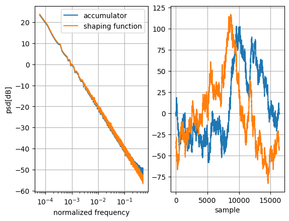
The accumulator is driven with the same input signal used for the frequency-domain filter. The figure below compares the magnitude of their outputs’ PSD and their over-time behavior. The PSD magnitude shows a similar \(1/f^2\) response for both, whereas the time-domain signals look different. The two signals in the time domain have approximately the same amplitude, but the similarities end there.
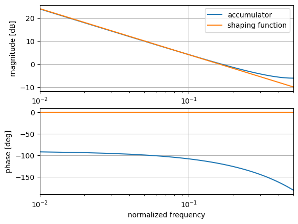
The missing piece of information can explain these differences: the phase of the signals. Comparing the transfer functions of both filters in the frequency domain reveals the source of the difference. The transfer function of the frequency-domain filter is the shaping function itself. The transfer function of the accumulator in the z-domain is:
\[H(z) = \frac{z^{-1}}{1-z^{-1}}\]The magnitude of its transfer function in the frequency domain then can be written as:
\[\left|H(j\omega)\right| = \left|\frac{e^{-j\omega T_s}}{1-e^{-j\omega T_s}}\right|\]The magnitude and phase responses for these transfer functions are plotted in the figure below. The accumulator shows a 90-degree phase shift at DC, which drops to 180 degrees at around \(f_s/2\). On the other hand, the frequency-domain filter shows a 0-degree phase shift across the entire band. Different frequency components are delayed differently for the accumulator, whereas the frequency-domain filter retains the phase of its input.
The second, and the less significant, difference originates from the time-domain accumulator’s behavior around frequencies close to \(f_s/2\). The accumulator does not maintain a \(1/f^2\) slope after its unity-gain frequency at \(f_s/6\), and the magnitude of its transfer function is 0.5 at \(f_s/2\).
Issues with Frequency-Domain Filtering
One might argue that frequency-domain filtering and time-domain filtering are equivalent. One could take the IDFT of the shaping function to get its impulse response and build a convolutional filter with it. Such an approach is entirely correct. The only difference between the two would be that the implementation is more efficient when utilizing the FFT.
The most prominent issue with this method is that it requires precomputing the entire noise signal. All samples that will be used must be computed before the start of the simulation and stored in memory. It is possible to quickly run into issues in long simulations requiring several such signals. A time-domain filter will generally require much less memory but might be computationally demanding during simulation.
A related problem is that simulation time must be known a priori to generate colored noise via frequency-domain filtering. The generated signals should be long enough to cover the entire length of the simulation. It is not trivial to stitch two signals generated via this method and achieve the same frequency-domain behavior due to windowing effects. The technique works well on noise signals that do not show specific features over time. However, utilizing it for generic filtering applications runs into windowing issues [2] that result in poor time domain responses.
The last one is not necessarily a unique problem to frequency-domain filtering. The simulation time must be estimated while synthesizing time-domain filters to find the number of stages that maintain the spectra to low frequencies. However, it’s much easier to overdesign since time-domain filters have significantly smaller memory requirements.
The Code
You can find the code used to generate the plots on GitHub.
References
[1] Algorithm for high quality 1/f noise? on Computational Science StackExchange
[2] Why is it a bad idea to filter by zeroing out FFT bins? on Signal Processing StackExchange